How Graph Attention Networks Work

Graphs - A Quick Primer

Before we get to the fancy stuff, let's make sure we're on the same page about what a graph actually is. If you've taken a discrete math or data structures class, you've seen this before - but it's worth revisiting because the intuition matters.

A graph is really just two things:

• Nodes (also called vertices) - these are the "things" in your graph
• Edges - these are the connections between things

That's it. A graph is a collection of things and the relationships between them.

Why Graphs Matter

Here's what took me a while to appreciate: graphs are everywhere. Once you start looking for them, you see them in everything:

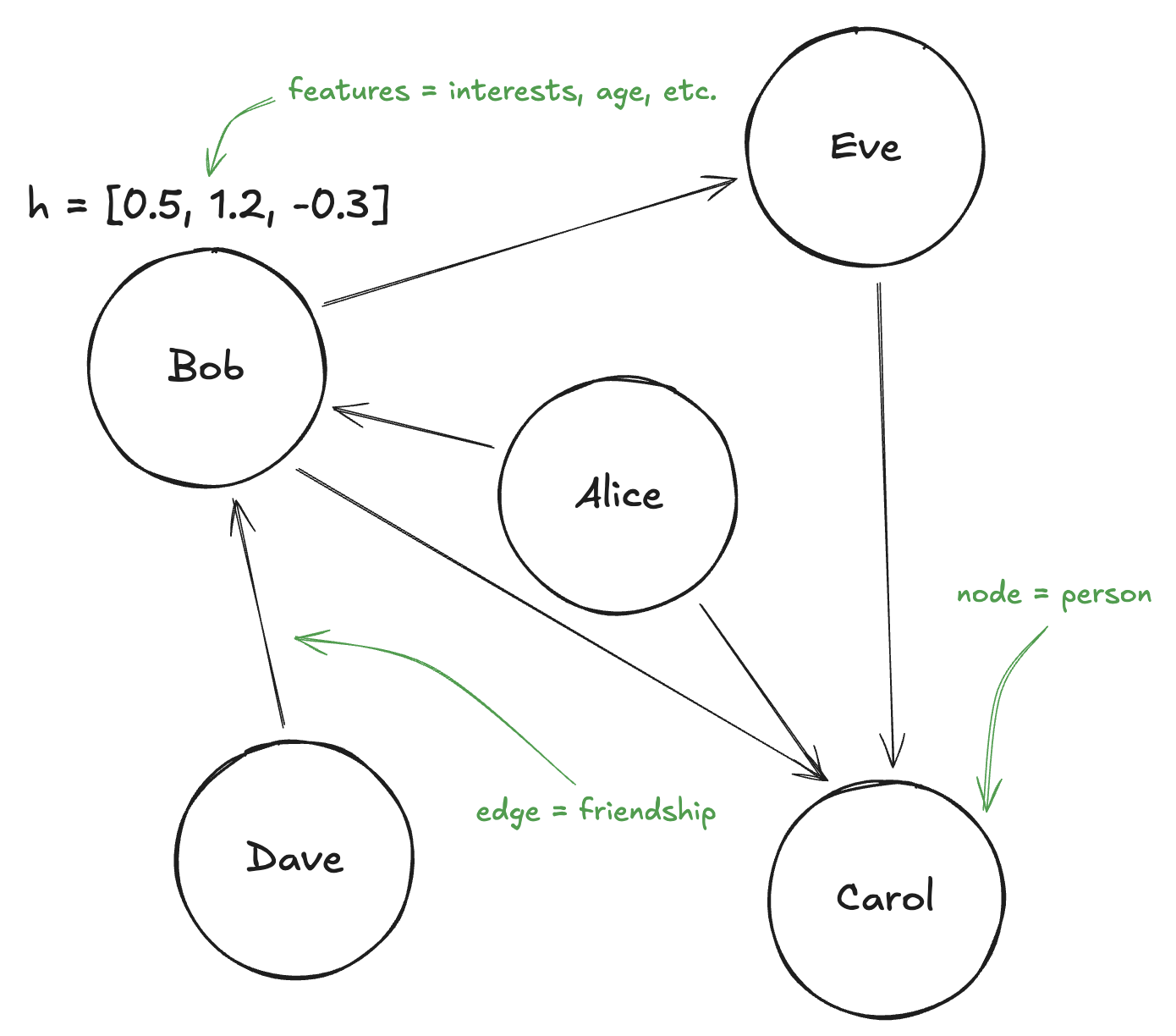
• Social networks: People are nodes, friendships are edges. Facebook's entire business is built on a graph.
• Molecules: Atoms are nodes, chemical bonds are edges. This is huge for drug discovery.
• The internet: Web pages are nodes, hyperlinks are edges. This is literally how Google started - PageRank is a graph algorithm.
• Knowledge bases: Concepts are nodes, relationships are edges. "Albert Einstein" → "born in" → "Germany".
• Road networks: Intersections are nodes, roads are edges. Google Maps uses graph algorithms to find your route.
• Biological networks: Proteins are nodes, interactions are edges. Understanding these graphs could help cure diseases.

The point is: a lot of real-world data naturally has this structure where you have entities and relationships between them. And if we want machine learning to work on this kind of data, we need neural networks that understand graphs.

Node Features

Here's something crucial: in machine learning on graphs, each node typically has features. These are just numbers that describe that node.

Think about a social network. Each person (node) might have features like:

• Age
• Number of posts per week
• Interests encoded as a vector
• Location (encoded somehow)

We typically represent a node's features as a vector $h_i$ - just a list of numbers. So node 1 might have features $h_1 = [0.5, 1.2, -0.3, ...]$, node 2 might have $h_2 = [0.8, 0.1, 0.9, ...]$, and so on.

The goal of a graph neural network is to learn better representations of these nodes - representations that capture not just the node's own features, but also information about its neighborhood.

This brings us to the key question: how do we actually process graph-structured data with neural networks?

The Problem with Regular Neural Networks

Here's the thing - you can't just throw graph data into a standard neural network. Let me explain why.

Regular neural networks expect inputs with a fixed structure:

• Images are always grids of pixels (say, 224 × 224 × 3)
• Audio is a sequence of samples at a fixed rate
• Text, after tokenization, is a sequence of token IDs

The network architecture is built around this fixed structure. A CNN expects a grid. An RNN expects a sequence. The weights are shaped to match.

But graphs? Graphs are messy:

• Variable size: Different graphs have different numbers of nodes
• Variable connectivity: Different nodes have different numbers of neighbors
• No natural ordering: There's no "first" node or "second" node. Who's first in a social network?
• Permutation invariance: The same graph can be represented in many equivalent ways just by relabeling the nodes

Imagine trying to flatten a social network into a fixed-size input vector. What if you have 1000 friends? What if you have 10? What order do you put them in? It just doesn't work.

This is where Graph Neural Networks (GNNs) come in. They're specifically designed to handle this variable, orderless structure.

Message Passing - The Core Idea

Okay, here's the big insight that makes GNNs work. It's called message passing, and once you understand it, everything else falls into place.

The intuition is simple: to understand a node, look at its neighbors.

Let me give you a concrete example. Imagine you're at a huge party and you don't know anyone. You want to figure out what kind of person someone is. What do you do?

You look at who they're hanging out with.

If all their friends are talking about startups and venture capital, they're probably into the startup world. If their friends are all musicians, they're probably into music. If they're surrounded by academics discussing research, they're probably an academic.

The people around you say something about you. Your social context is informative.

GNNs formalize this exact intuition. In each layer of a GNN, every node:

1. Collects "messages" from its neighbors - basically, it looks at their feature vectors
2. Aggregates these messages - combines them somehow (we'll talk about how)
3. Updates its own representation - incorporates this neighborhood information

This happens for every node in parallel. Then we repeat for multiple layers. After a few layers, each node's representation captures information not just from its immediate neighbors, but from neighbors of neighbors, and so on.

The Aggregation Problem

So here's the question: how do you actually aggregate messages from neighbors?

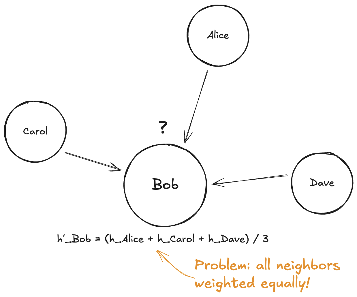
The simplest approach is to just average them. If node $i$ has neighbors $j_1, j_2, j_3$, its new representation is just:

Where $\mathcal{N}_i$ is the set of neighbors of node $i$, and $|\mathcal{N}_i|$ is how many neighbors there are.

In plain English: add up all your neighbors' feature vectors, then divide by the number of neighbors.

This works! And simple averaging-based GNNs can be pretty effective. But there's a problem.

All neighbors are treated equally.

Let's go back to the party analogy. Imagine you want career advice. You could ask:

• Your best friend who knows you really well and has great judgment
• A random person you just met five minutes ago
• That guy who keeps giving terrible advice and doesn't really understand you

Would you weight their opinions equally? Of course not! Your best friend's advice is probably way more valuable than the random stranger's.

But simple averaging treats them all the same. It doesn't distinguish between highly relevant neighbors and barely relevant ones.

Some neighbors are more relevant than others. We need a way to learn which ones matter more.

Enter Attention - "Who Should I Listen To?"

This is exactly what attention gives us. Instead of treating all neighbors equally, we learn attention weights that determine how much each neighbor contributes.

Building the Intuition

Let's stick with the party analogy because I think it really helps here.

When you're at a party, you naturally pay more attention to some people than others. Think about what affects how much attention you give someone:

• Similarity: You lean in more when someone shares your interests
• Relevance: If you're thinking about career stuff, you pay more attention to people who can help with that
• Trust/Familiarity: You weight your close friend's opinion more than a stranger's
• Expertise: You listen more to people who know what they're talking about

You don't consciously decide "I'm going to weight Alice at 0.4 and Bob at 0.1." But your brain is doing something like that automatically.

GATs learn to do the same thing. Given a node and its neighbors, the network learns to assign attention weights that reflect "how much should I listen to this neighbor?"

What Attention Gives Us

For each node $i$ and each of its neighbors $j$, GAT computes an attention weight $\alpha_{ij}$. These weights have some nice properties:

• They're learned: The network figures out what makes a neighbor "important" during training. We don't hand-code the rules.
• They're normalized: The weights across all neighbors sum to 1. So they're like a probability distribution - "what fraction of my attention goes to each neighbor?"
• They're dynamic: The weight depends on both the node and its neighbor, not just the graph structure. Same neighbor might get different attention from different nodes.

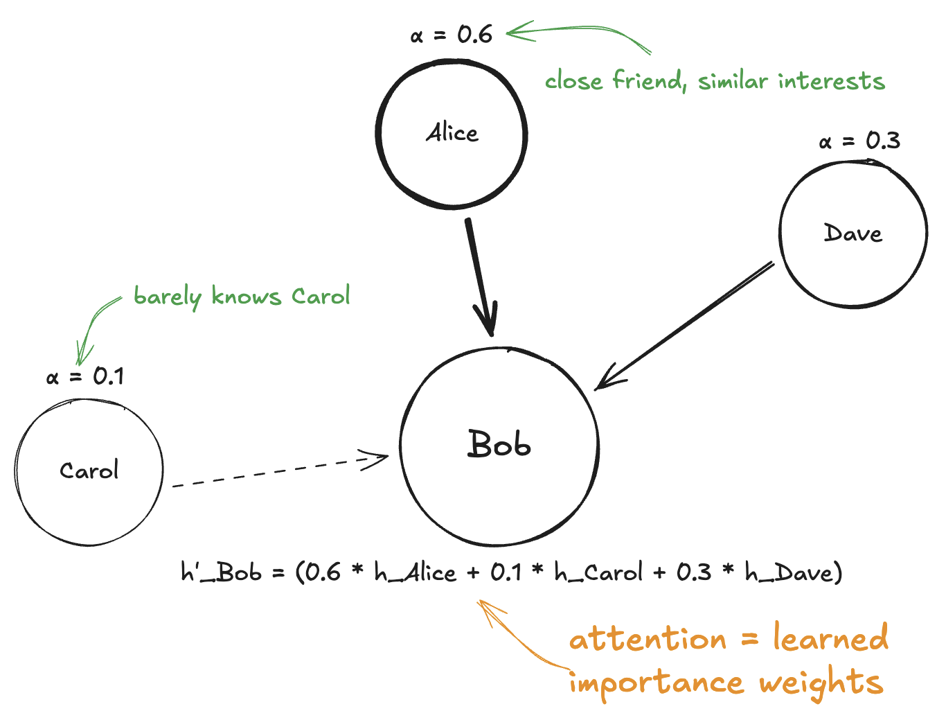
Now instead of simple averaging, we compute a weighted sum:

Let's break this down:

• $h'_i$ is the new representation for node $i$ (the output)
• We sum over all neighbors $j$ in the neighborhood $\mathcal{N}_i$
• Each neighbor's features $h_j$ are multiplied by their attention weight $\alpha_{ij}$

So if Alice has weight 0.6, Dave has weight 0.3, and Carol has weight 0.1, the new representation is:

Bob's new representation is mostly influenced by Alice, somewhat by Dave, and barely by Carol. That's the power of attention.

But here's the million-dollar question: where do these attention weights actually come from?

The GAT Mechanism

Alright, now we get to the heart of how GAT actually works. I'm going to walk through this step by step, showing both the math and the intuition. Don't worry if the math looks intimidating at first - I'll explain every piece.

The high-level idea is:

1. Transform node features into a new space
2. Compute a "compatibility score" for each pair of connected nodes
3. Normalize these scores into proper weights
4. Use the weights to aggregate neighbor information

Let's go through each step.

Step 1: Transform the Features

First, we apply a linear transformation to each node's features. This is just matrix multiplication:

Let's unpack this:

• $h_i$ is the original feature vector for node $i$ (say, a vector of length $F$)
• $W$ is a learnable weight matrix (size $F' \times F$)
• $z_i$ is the transformed feature vector (length $F'$)

Why do we do this? A few reasons:

• Change dimensionality: We might want to project into a smaller or larger space
• Learn what matters: The matrix $W$ learns to emphasize features that are important for the task
• Create a common space: Before comparing two nodes, we want their features in the same "language"

Think of it like this: before comparing two people at a party, you first translate everyone's profile into a standardized format that highlights the things that matter for your comparison.

Key point: The same matrix $W$ is applied to every node. This is important for making the network efficient and ensuring it generalizes.

Step 2: Compute Attention Scores

Now comes the clever part. We need to compute how much node $i$ should "attend to" node $j$.

The intuition is: we want to measure "compatibility" between two nodes. Are their features such that $j$ would be helpful for $i$?

GAT does this in a specific way:

1. Take the transformed features of both nodes: $z_i$ and $z_j$
2. Concatenate them: stack them together into one longer vector $[z_i \| z_j]$
3. Pass this through a learnable "attention mechanism"
4. Apply a non-linearity

In math:

Let me explain each piece:

The concatenation $[z_i \| z_j]$: We're just stacking the two vectors. If $z_i$ has length $F'$ and $z_j$ has length $F'$, then $[z_i \| z_j]$ has length $2F'$.

The attention vector $\mathbf{a}$: This is the second set of learnable parameters (after $W$). It's a vector of length $2F'$. When we compute $\mathbf{a}^T \cdot [z_i \| z_j]$, we're taking a dot product - this gives us a single number.

What does this dot product mean intuitively? The vector $\mathbf{a}$ learns a kind of "compatibility function." It learns which combinations of features between node $i$ and node $j$ indicate that $j$ is relevant to $i$.

The LeakyReLU: This is a non-linearity. Regular ReLU sets all negative values to zero:

LeakyReLU instead lets a small fraction of negative values through:

Why LeakyReLU? It helps with training stability. If we used regular ReLU, some attention scores could get "stuck" at zero and never recover during training.

The output $e_{ij}$ is called the raw attention score. It's a single number that represents "how compatible are nodes $i$ and $j$?"

But we're not done yet. These raw scores could be any real number - positive, negative, large, small. We need to turn them into proper weights.

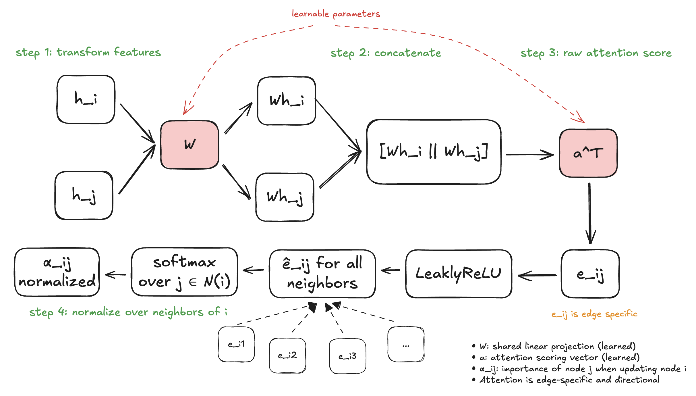
Step 3: Normalize with Softmax

We have raw scores $e_{ij}$ for each neighbor. Now we need to convert them into proper attention weights that:

1. Are all positive (you can't have negative attention)
2. Sum to 1 across all neighbors (so they're like a probability distribution)

The standard way to do this is softmax:

Let me break this down, because softmax trips people up:

• The numerator $\exp(e_{ij})$ is $e$ raised to the power of $e_{ij}$. This makes everything positive.
• The denominator sums this over ALL neighbors $k$ of node $i$. This normalizes so everything sums to 1.

Let's work through a concrete example. Say node $i$ has three neighbors with raw scores:

• $e_{i,\text{Alice}} = 2.0$
• $e_{i,\text{Carol}} = 1.0$
• $e_{i,\text{Dave}} = 0.5$

First, we compute $\exp$ of each:

• $\exp(2.0) \approx 7.39$
• $\exp(1.0) \approx 2.72$
• $\exp(0.5) \approx 1.65$

The sum is $7.39 + 2.72 + 1.65 = 11.76$

So the attention weights are:

• $\alpha_{i,\text{Alice}} = 7.39 / 11.76 \approx 0.63$
• $\alpha_{i,\text{Carol}} = 2.72 / 11.76 \approx 0.23$
• $\alpha_{i,\text{Dave}} = 1.65 / 11.76 \approx 0.14$

Notice: $0.63 + 0.23 + 0.14 = 1.0$. The weights sum to 1, as promised.

Softmax has a nice property: it amplifies differences. Alice's raw score was only twice Dave's (2.0 vs 0.5), but her attention weight is more than four times larger (0.63 vs 0.14). The exponential function makes the highest scores dominate.

Step 4: Aggregate

Finally! We have our attention weights $\alpha_{ij}$. Now we just use them to compute a weighted sum:

Breaking this down:

• For each neighbor $j$, take their transformed features $z_j$
• Multiply by the attention weight $\alpha_{ij}$
• Sum all these up
• Apply a non-linearity $\sigma$ (often ReLU or ELU)

The result $h'_i$ is the new representation for node $i$. It's a combination of its neighbors' information, but weighted by how much $i$ should "attend to" each one.

Putting It All Together

Let's recap the full GAT layer. Given node $i$ with neighbors $\mathcal{N}_i$:

1. Transform: $z_i = W \cdot h_i$ for all nodes
2. Score: $e_{ij} = \text{LeakyReLU}(\mathbf{a}^T [z_i \| z_j])$ for all edges
3. Normalize: $\alpha_{ij} = \text{softmax}_j(e_{ij})$
4. Aggregate: $h'_i = \sigma(\sum_j \alpha_{ij} z_j)$

The learnable parameters are:

• $W$ - the feature transformation matrix (learns what features matter)
• $\mathbf{a}$ - the attention vector (learns what makes nodes compatible)

During training, backpropagation adjusts both $W$ and $\mathbf{a}$ to minimize your loss function. The network learns both what features are important AND how to compute compatibility between nodes.

That's the core GAT mechanism! But there's one more trick that makes it work even better.

Multi-Head Attention

Here's a question that might have occurred to you: what if different types of "importance" matter in different ways?

Why Multiple Heads?

Think about what makes a neighbor "relevant." There could be many reasons:

• Maybe they're structurally similar (same number of connections)
• Maybe they have similar features
• Maybe they're in the same community
• Maybe they have complementary information

A single attention mechanism (one $W$ and one $\mathbf{a}$) might not capture all these different notions of relevance.

The solution is multi-head attention. Instead of computing one set of attention weights, we compute $K$ independent sets, each with its own parameters.

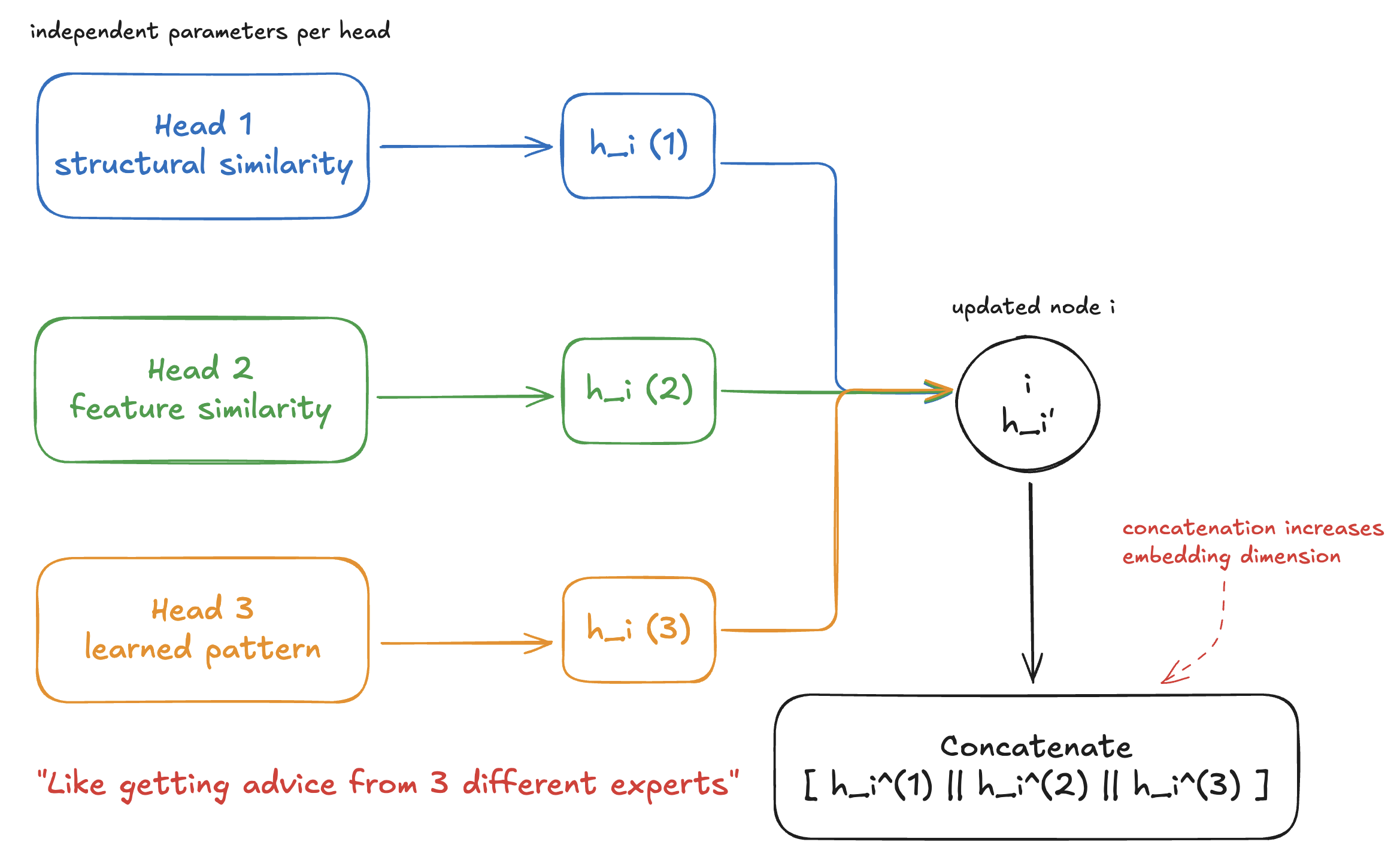
Think of it like consulting multiple experts:

• Expert 1 focuses on one aspect of the problem
• Expert 2 focuses on a different aspect
• Expert 3 focuses on yet another aspect

By combining their perspectives, you get a richer understanding than any single expert could provide.

In math, we have $K$ attention heads, each computing:

Where the superscript $(k)$ indicates the $k$-th head, each with its own $W^{(k)}$ and $\mathbf{a}^{(k)}$.

We then combine the outputs from all heads. Typically, we concatenate them:

Where $\|$ means concatenation. If each head outputs a vector of length $F'$, and we have $K$ heads, the final output has length $K \cdot F'$.

For the final layer of the network, we often average instead of concatenate, to get a fixed output size:

In practice, 4 to 8 attention heads is common. More heads = more expressive power, but also more parameters and computation.

Multi-head attention also helps stabilize training. If one head learns something weird, the others can compensate. It's like having multiple independent "votes" on what's important.

Importance vs. Correlation

Now for a question that bugged me for a while: is attention actually learning which neighbors are "important"? Or is it learning something else?

The honest answer is: it's complicated.

What attention is actually doing: it's learning which neighbors have features that are useful for the task you're training on.

Let me make this concrete. Say you're training a GAT to classify nodes in a social network as "will churn" or "won't churn" (i.e., will they stop using the service).

The attention mechanism learns: "which of my neighbors' features are predictive of whether I'll churn?"

This might align with human intuition about "importance":

• Maybe close friends who have churned are highly predictive → high attention
• Maybe acquaintances you barely interact with are less predictive → low attention

But it might not always match our intuition:

• Maybe a seemingly "unimportant" neighbor is actually highly predictive because they provide unique information
• Maybe attention is spread evenly because many neighbors are equally informative
• Maybe the model learns spurious correlations in the training data

The key insight: attention weights are task-dependent. They're not an objective measure of "importance" - they're a learned measure of relevance for the specific thing you're trying to predict.

This is actually a common point of confusion with attention mechanisms in general (including in transformers for NLP). High attention weight doesn't necessarily mean "important" in a human-intuitive sense. It means "useful for reducing the loss function."

That said, attention weights can still be useful for interpretability - they give you some signal about what the model is looking at. Just don't over-interpret them.

When GATs Struggle

GATs are powerful, but they're not magic. Let me walk you through the main failure modes so you know what to watch out for.

1. Over-smoothing

This is probably the biggest issue with GNNs in general, not just GATs.

Remember how message passing works: each layer aggregates information from neighbors. After one layer, each node knows about its 1-hop neighbors. After two layers, it knows about 2-hop neighbors. And so on.

The problem: as you stack more layers, node representations start to converge. Everyone starts looking the same.

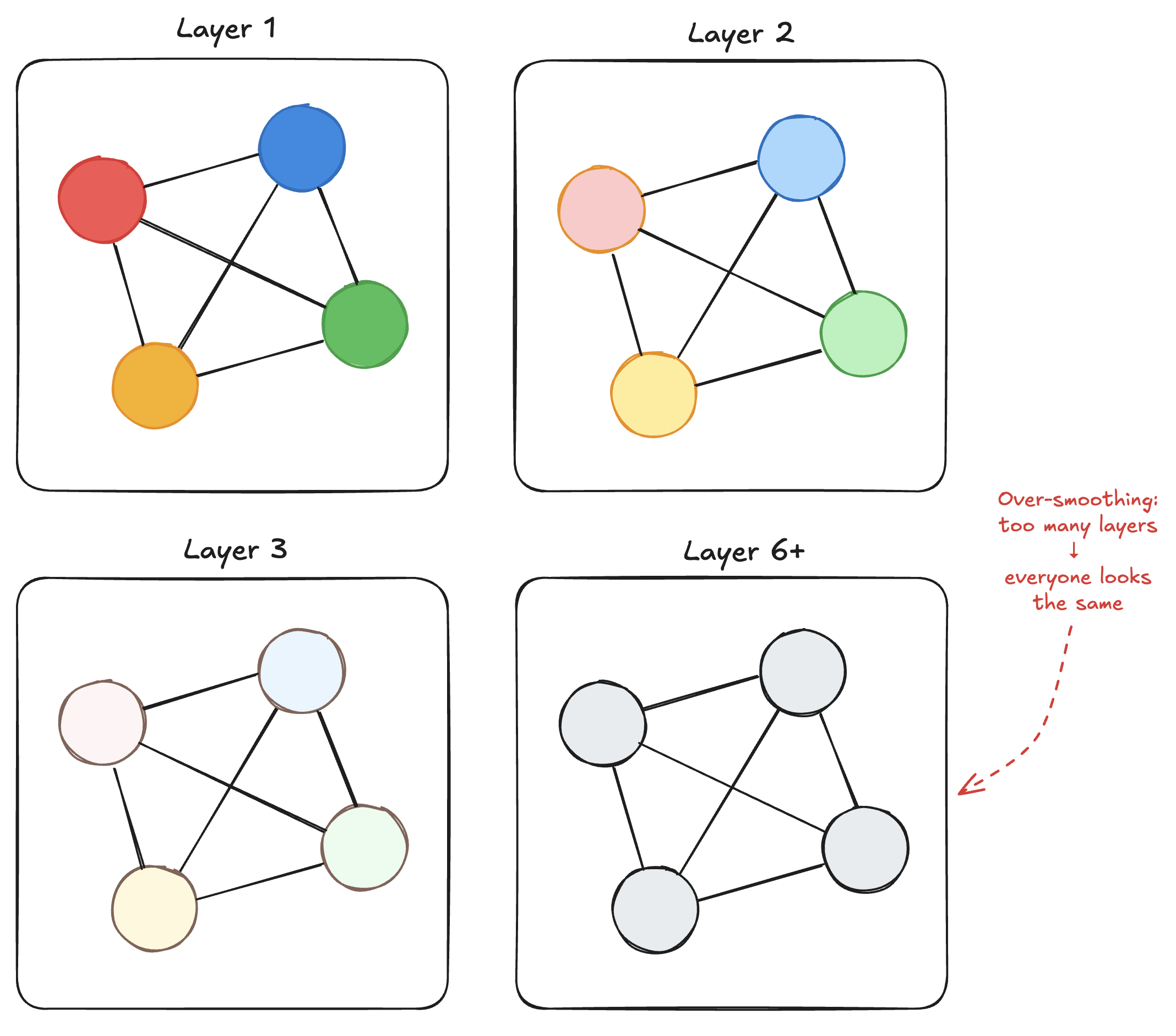
It's like a game of telephone. After enough rounds of passing messages, everyone's heard from everyone else, and individual differences wash out.

This limits how deep you can make your GNN. While CNNs can be hundreds of layers deep, GNNs typically use 2-4 layers before over-smoothing becomes a problem.

There are techniques to mitigate this (residual connections, normalization, etc.), but it's an active area of research.

2. Heterogeneous Graphs

What if your graph has different types of nodes or edges?

For example, in a knowledge graph: "Einstein" (person) → "born_in" → "Germany" (country) → "located_in" → "Europe" (continent). You have different node types and different edge types.

A single GAT attention mechanism might struggle here. The same "compatibility function" might not make sense for all edge types. Why would "born_in" relationships have the same attention pattern as "located_in" relationships?

Variants like Heterogeneous Graph Attention Networks (HAN) address this by having separate attention mechanisms for different edge types.

3. When Neighbors Genuinely Don't Vary in Importance

Sometimes, all your neighbors really are equally important.

In these cases, learning attention weights adds parameters without benefit. You're essentially learning to approximate uniform weighting - but with extra steps and extra parameters.

If your task doesn't benefit from differentiated attention, simpler GNNs (like GCN) might actually work better - fewer parameters, faster training, less overfitting risk.

4. Computational Cost

Computing attention scores requires looking at every edge in the graph. For each edge, we do a concatenation and a dot product.

For large, dense graphs, this can be expensive. If you have millions of nodes and billions of edges, those attention computations add up.

There are approximations and sampling techniques to make this more tractable, but it's worth being aware of the cost.

Conclusion

Let's recap what we've learned:

• Graphs are everywhere - social networks, molecules, knowledge bases - and they need special neural network architectures that respect their structure.
• Message passing is the core idea behind GNNs: understand a node by aggregating information from its neighbors.
• The aggregation problem: simple averaging treats all neighbors equally, but some neighbors are more relevant than others.
• Attention solves this by learning weights that reflect how much to "listen to" each neighbor.
• GATs compute attention by transforming features, computing compatibility scores, normalizing with softmax, and aggregating.
• Multi-head attention lets the model capture different notions of relevance simultaneously.
• Attention weights are task-dependent - they reflect what's useful for prediction, not necessarily human intuition about importance.
• GATs have limitations - over-smoothing, heterogeneous graphs, computational cost - that you should be aware of.

Working through GATs really helped me understand not just how they work, but why they're designed the way they are. The math is elegant, and the intuitions carry over to other attention-based architectures too.

If you're working with graph data - whether that's social networks, molecules, knowledge graphs, or something else entirely - GATs are a powerful tool to have in your toolkit. And now you actually understand what's happening under the hood.

Next up, I want to dig into some of the variants - like how Graph Transformers handle attention differently, or how heterogeneous graph networks extend these ideas to multi-relational data. But that's for another post.

If you found this helpful or have questions, feel free to reach out on Twitter. I'm always happy to chat about this stuff.